3. Graphical user interface manual
| Date: | February 17, 2017 |
|---|
This document aims to get you used to the gsimcli’s graphical user interface (GUI). It is divided into sections that more or less match the interface sections.
The interface was designed to be easy and intuitive to use, having a lot of common structures seen in other programs.
Contents
3.1. Overview
The main window is divided into four sections, as shown in the figure below:
- on top (depending on the operating system) there is the main menu;
- all the homogenisation process settings are accessed on the left menu;
- below the left menu, on the bottom left corner, there is the status box;
- the remaining area on the right is where the settings are shown.
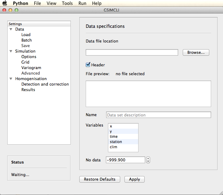
Overview of the graphical user interface
There are two auxiliary buttons on the main window:
- Apply will save the current settings.
- Restore Defaults will change all settings to the default values (not implemented yet).
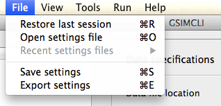
3.2. Main menu
The main menu includes a few other subsections. When available, the actions listed in the main menu may be followed by a keyboard shortcut, as illustrated in the Main menu example.
3.2.1. File
From here you can read and write files.
3.2.1.1. Restore last session
Reload all the settings used in the last session (if any).
3.2.1.2. Open settings file
Load all the settings saved into a configuration file. The file extension depends on your operating system and it should be automatically detected.
3.2.1.3. Recent settings files
List the last 10 configuration files which were opened or saved and it will load all the settings saved in the selected file.
3.2.1.4. Save settings
Save the current settings into the configuration file previously loaded.
Warning
it will not overwrite the settings file previously loaded, for that purpose you should use Export settings. This behaviour is expected to change in a future version.
3.2.1.5. Export settings
Save the current settings into a new configuration file.
3.2.1.6. Quit
Exit from the application.
3.2.2. View
3.2.2.1. Print status (console)
Enable or disable the program output into the console (terminal emulator). If any error occur while running the application, it will be printed in the console regardless of this option.
3.2.3. Tools
Not implemented yet.
3.2.4. Run
3.2.4.1. GSIMCLI
Start the homogenisation process with the current settings. The process progress will be stated in the status box.
3.2.5. Help
3.2.5.1. Online documentation
This is a link to the online documentation, which should open in your browser.
3.2.5.2. About
Some information about the application.
3.3. Settings
This GUI basically serves the purpose of preparing and launching the GSIMCLI homogenisation process. This process depends on several settings which are user adjustable.
There are three groups of settings for you to set up: Data, Simulation and Homogenisation.
3.3.1. Data
In this group you set up the data to be homogenised.
3.3.1.1. Load
Options to load a single data file and set the specifications of the chosen file (or of multiple files with the same format).
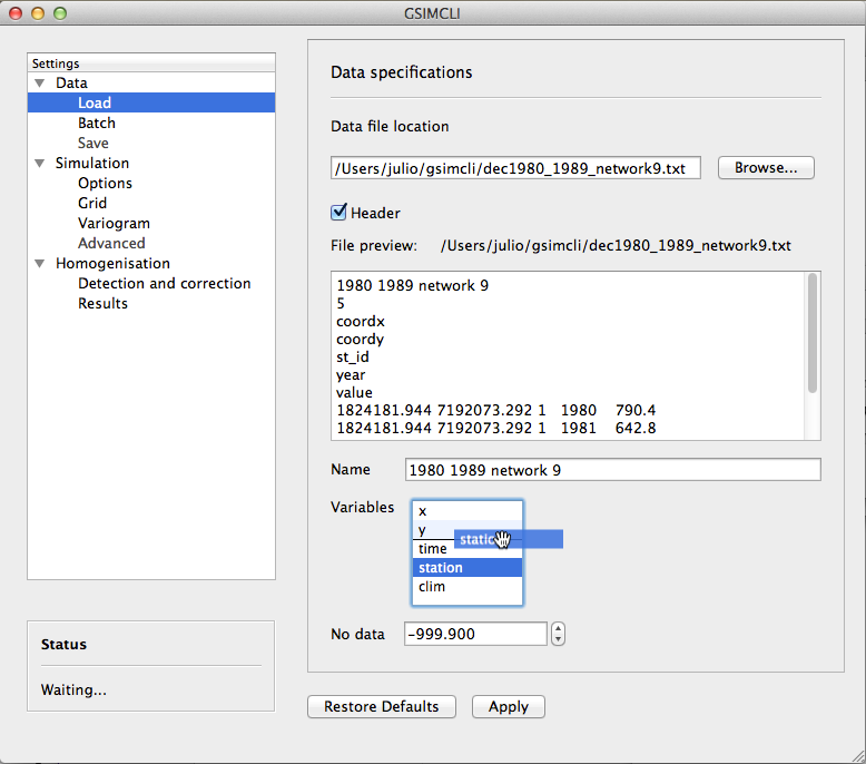
Example of the Data/Load settings pane
3.3.1.1.1. Data file location
Browse a single file containing the data set. This option is automatically disabled if Batch is enabled.
3.3.1.1.2. Header
Enable if every data file has header lines as the standard specified in the GSLIB format [1].
3.3.1.1.3. File preview
Show the first 10 lines of the loaded file. It is useful to double check the existence of header lines and the variables order.
When processing multiple networks, it will try to locate one of the data files of the selected network and display its first 10 lines.
3.3.1.1.4. Name
The data set name. If header is enabled, it will automatically extract the first line of the data file into this field, but it will remain editable.
3.3.1.1.5. Variables
Select the correct variables order, which should match the structure of the given data files. You can adjust their order through drag and drop. There are five default variables that your data file should include:
| x: | value for the X-coordinate. |
|---|---|
| y: | value for the Y-coordinate. |
| time: | value for the unit of time (e.g., year). |
| station: | the station ID number. |
| clim: | value for the climate variable. |
The previous example shows the preview of a loaded data file and the matching (drag and drop) of the variable corresponding to the station ID.
3.3.1.1.6. No data
The numeric placeholder for missing data. The default value is -999.9.
3.3.1.2. Batch
Depending on the size of the data set and on the selected settings, the homogenisation process may take a few hours or even several days. These batch options allow you to prepare different networks and leave them to run as on a queue list.
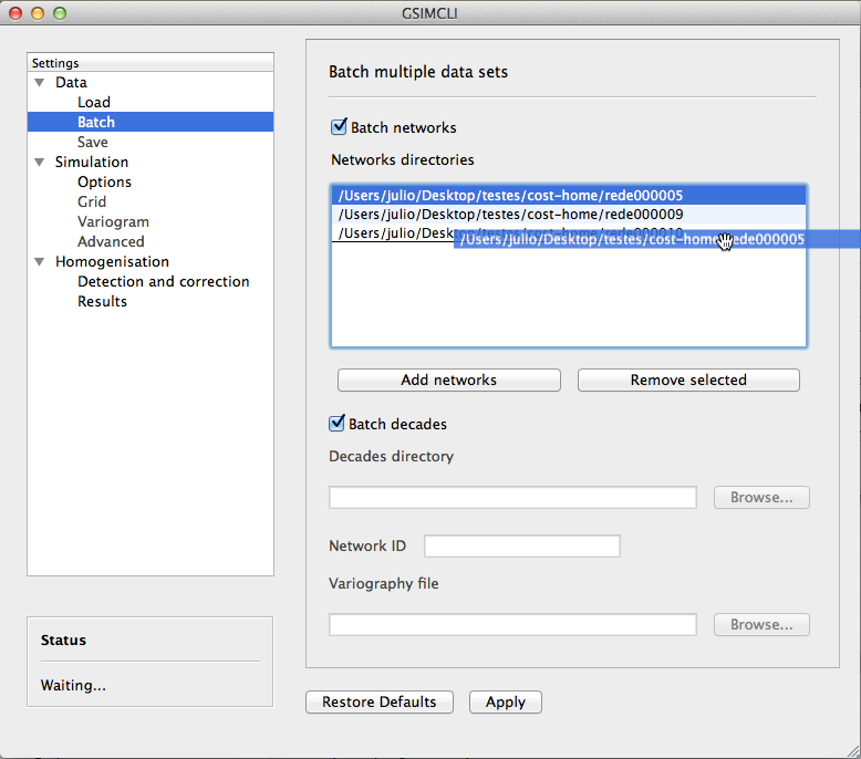
Example of the Data/Batch settings pane
In this example, three networks were selected and the order in which they are going to be homogenised is being changed (the network rede000005 will be the last one).
The options below Batch decades are grayed out because Batch networks is enabled.
3.3.1.2.1. Batch networks
This option allows you to select multiple networks to homogenise. Each network data set must follow a specific format and must have a main folder with a (meaningful) identification name/number, which contains:
- a file with the grid properties, this file name must be of the type
*grid*.csv; - as of version 0.0.1, it is mandatory that Batch decades is enabled and thus its requirements must also be followed;
- a folder which name starts with
*dec*(e.g., decades or dec_files); - a variogram file within it, and this file name must be of the type
*variog*.csv.
The file with the grid properties must follow these specifications:
comma separated values (CSV)
seven labelled columns (not case sensitive):
- xmin: initial value in X-axis
- ymin: initial value in Y-axis
- xnodes: number of nodes in X-axis
- ynodes: number of nodes in Y-axis
- znodes: number of nodes in Z-axis
- xsize: node size in X-axis
- ysize: node size in Y-axis
- other columns will be ignored
After enabling this option, the buttons to add and remove networks become available.
Press the button Add networks to select the main directories of the networks to be homogenised. You can select multiple folders (networks) at the same time by pressing CTRL (PC) or CMD (Mac) while selecting them.
After adding networks to the queue list, you can remove one or multiple networks from the list by selecting them and pressing the button Remove selected. Also, if you select one of the networks in that list, one of its data files will be previewed in the File preview area.
It is also possible to change the order in which the networks will be processed by drag and dropping from the list, as seen in the Example of the Data/Batch settings pane.
Note
when Batch networks is enabled, the settings menu to set up the simulation Grid automatically becomes unavailable, you have to specify the grid through a spreadsheet file.
Warning
it is only working if Batch decades is also enabled. For that reason, the grid is assumed to have 10 nodes of size 1 in the Z-axis (10 years).
3.3.1.2.2. Batch decades
It might be useful to process a time series in chunks of time, for instance, if your data set spans a full century, splitting the data in decades may help to analyse local (temporal) trends or irregularities, or it just can ease the computational weight.
In order to enable this option, the following requirements must be followed:
- your data set files must be placed inside the folder;
- the decadal data files must have, at least, the first year of each decade in their file names;
- you should provide a spreadsheet file with the theoretical variogram model.
The variograms file must follow these specifications:
comma separated values (CSV)
nine labelled columns (not case sensitive):
- variance: the data variance per decade
- decade: decade in the format aaXX-aaYY (aa is optional)
- model: ‘S’, ‘E’ or ‘G’ (S = spherical, E = exponential, G = gaussian)
- nugget: nugget effect
- range the variogram range
- partial sill
- nugget_norm: variance-normalised nugget effect
- psill_norm: variance-normalised partial sill
- sill_norm: variance-normalised total sill
- other columns will be ignored
Note
The variogram is assumed to be isotropic in the horizontal direction and with range 1 (one unit) in the vertical (time) direction. It will default its angles to (0, 0, 0).
After enabling this option, the related areas become available, except if Batch networks is also enabled, in which case it is not necessary to specify anything else.
If not processing multiple networks, the following fields must be filled:
- Decades directory: the folder containing your decadal files.
- Network ID: the network ID name/number. The program will try to guess the ID from the decades directory, but you can change it after that.
- Variography file: the spreadsheet file containing the variogram model.
Note
when Batch decades is enabled, the settings’ menu to set up the Variogram automatically becomes unavailable, you have to specify the variogram through a spreadsheet file.
3.3.2. Simulation
The gsimcli homogenisation process is based on a geostatistical stochastic simulation method. It is necessary to specify several options related to that part of the process, however, a set of default values are provided in the GUI. Also, the less relevant [to the homogenisation process] simulation parameters are conveniently hidden and placed in a section for Advanced settings.
3.3.2.1. Options
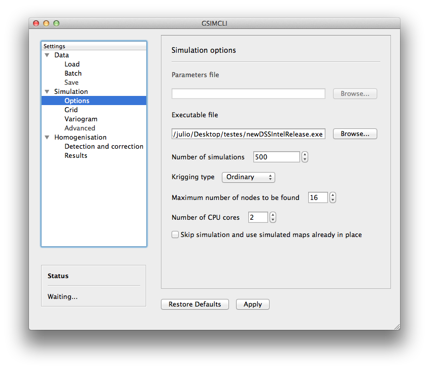
Example of the Simulation/Options settings pane
3.3.2.1.1. Parameters file
The simulation parameters file, in its original format. As of version 0.0.1, that file will be automatically generated, and this field is disabled.
3.3.2.1.2. Executable file
The simulation (Direct Sequential Simulation – DSS) binary file. As of version 0.0.1, only the 2001 version is supported. You can get the binary from the CMRP Software [2] site. Download the file GeoMS.zip and extract the binary dssim.exe.
3.3.2.1.3. Number of simulations
The number of simulations per candidate station. A brief study demonstrated that a higher number leads to better results, as it will produce a smoother local distribution. A low number (below 100) will produce a distribution with artifacts, while a number too high will require too much CPU time. We advise you to run the process with a few hundreds (e.g., 500) realisations per candidate station.
3.3.2.1.4. Krigging type
The krigging estimator used while simulating each node:
- Ordinary (OK)
- Simple (SK)
3.3.2.1.5. Maximum number of nodes to be found
Related to the search method.
We advise the value 16, in the range 1 – 64. A higher number will produce a better spatial correlation in the simulated maps but it will demand an unnecessary higher computational effort. We found that a value above 16 would not bring enough benefits to justify the increasing CPU time.
The remaining parameters related to the search method are defined by default, as we tested them and found these values to be a good starting point. Those parameters are:
- Search strategy: data nodes (do not search for real and simulated data separately).
- Grid search method: spiral search (search for the nearest nodes according to a spiral pattern).
- Search radius: equal to the given grid dimensions.
- Number of samples, Samples per octant, and Search angles, are irrelevant for the data nodes search strategy.
3.3.2.1.6. Number of CPU cores
Recent computers often have multiple central processing units (CPU’s) or one CPU with multiple cores, where each of them can be assigned to run a different process at the same time.
In this program, such technology can be used to speed up the overall process. Specifically, you can opt to run multiple simulations at the same time if your computer has that capability, instead of running one at a time.
The program will detect the number of cores installed and select that value by default. In the Example of the Simulation/Options settings pane, the program detected the maximum number of 2, which corresponds, in this case, to a CPU with two processor cores.
Note
The parallelised DSS version is not supported. The multi-threading is attained through a script that will prepare and launch a number of copies of the DSS binary equal to the given number of CPU cores, which, in fact, may be more efficient than the parallelised version, because only some specific parts of the algorithm will run in parallel mode.
3.3.2.1.7. Skip simulation and use simulated maps already in place
Enable this option if you have already run all the simulations and have kept the resulting maps in the results folder.
This option is useful for debugging purposes or if you need to rebuild the results file.
3.3.2.2. Grid
Here you specify the simulation grid:
- Grid dimension: the number of nodes/cells in each direction.
- Cell size: the length (in units of distance) of one side of each cell (which are squared).
- Origin coordinates: the position (in units of distance) of the first cell.
Note
The Z-axis corresponds to time.
This section will be automatically disabled when Batch networks is enabled.
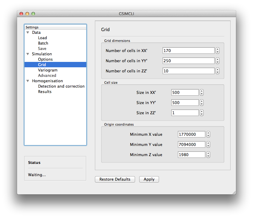
Example of the Simulation/Grid settings pane
 nodes, covering a total area of
 units of area. That
time series spans the decade of 1980 to 1989 (10 nodes of size 1 in the
Z-axis).
units of area. That
time series spans the decade of 1980 to 1989 (10 nodes of size 1 in the
Z-axis).3.3.2.3. Variogram
In this screen there are the necessary fields to set up the theoretical variogram model:
- Model (Spherical, Exponential or Gaussian)
- Nugget effect (normalised)
- Sill (normalised)
- Ranges (three comma separated values)
- Angles (three comma separated values)
This section will be automatically disabled when Batch decades is enabled.
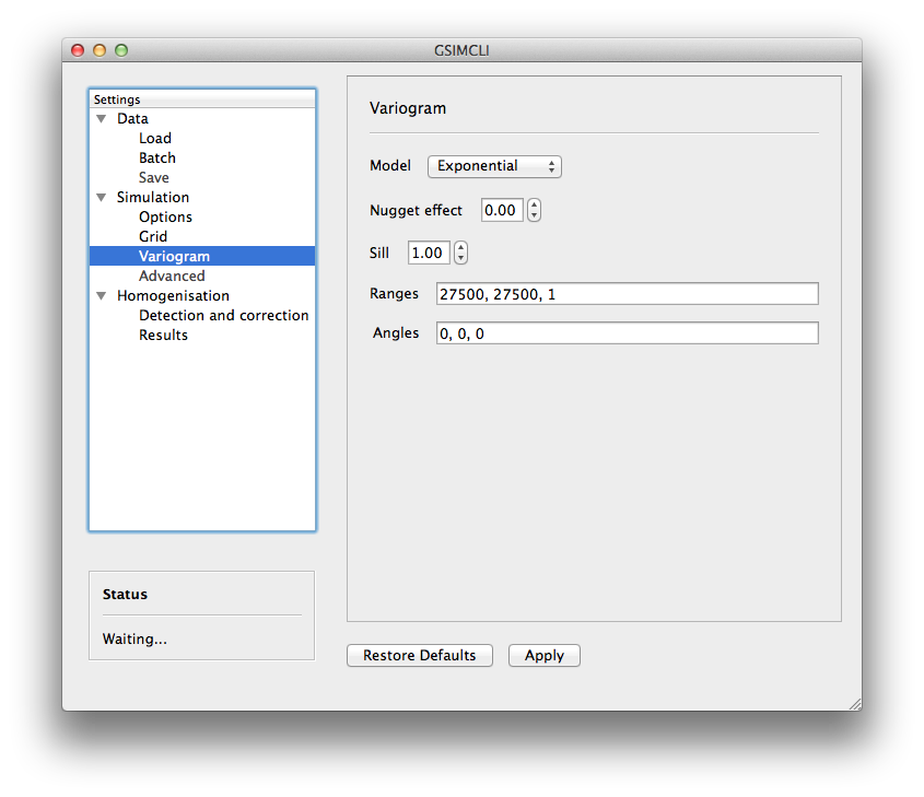
Example of the Simulation/Variogram settings pane
3.3.2.4. Advanced
Options to change the remaining DSS parameters. Not implemented yet.
3.3.3. Homogenisation
The homogenisation process may be divided into two major steps: the detection of irregularities and then their correction.
In gsimcli method, the simulation plays an import role in the detection of irregularities, but there are a few more parameters that can be adjusted, regarding on the way the simulation is embedded in the homogenisation process.
3.3.3.1. Detection and correction
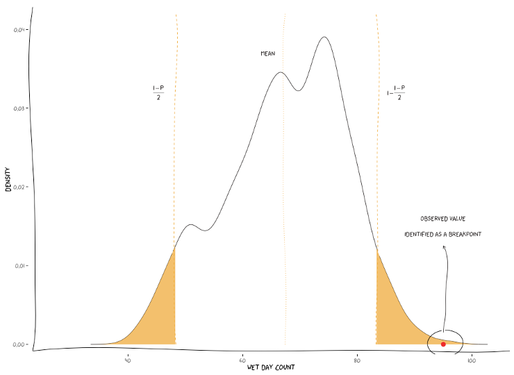
A breakpoint is identified whenever the interval of a specified probability p (e.g., 0.95), centred in the local PDF, does not contain the observed (real) value of the candidate station. In practice, the local PDF’s are provided by the histograms of simulated maps. Thus, this rule implies that if the observed (real) value lies below or above the predefined percentiles of the histogram, of a given instant in time, then it is not considered homogeneous.
If irregularities are detected in a candidate series, the time series can be adjusted by replacing the inhomogeneous records with the mean, or median, of the PDF(s) calculated at the candidate station’s location for the inhomogeneous period(s) [COSTA2009] (with time, different methods of correction may be introduced).
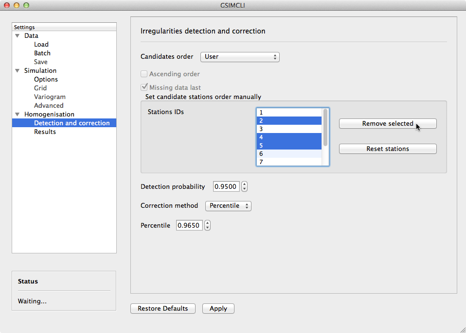
Example of the Homogenisation/Detection and correction settings pane
3.3.3.1.1. Candidates order
The order in which the candidates stations will be homogenised. There are a few options to arrange all stations in different manners, or you can provide your own arrangement.
The available options to sort the candidate stations are:
- ID order: according to the stations’ ID name/number.
- Network deviation: according to the difference between the station average and the network average.
- Random: all stations randomly sorted.
- Variance: sorts all stations by greater or lower variance.
- User: the user specifies which stations will be homogenised and their order.
If you select User, the stations’ IDs will be automatically detected and listed. Then, you can reorder them by drag and drop, remove any that is not to be homogenised by pressing Remove selected, or reset the list to its original state by pressing Reset stations (see the example above).
Note
That stations list will only appear if you have enabled Batch networks and only one network have been added.
3.3.3.1.2. Ascending order
You also can specify if this sorting is done in ascending or descending order. For instance, for the Variance sorting method, if you disable Ascending order, it will sort all stations by greater variance (which is the default option).
3.3.3.1.3. Missing data last
If a station has no data in the time period being processed, you can opt to homogenise that station in the first place, or only after the remaining candidate stations.
3.3.3.1.4. Detection probability
Probability value to build the detection interval centred in the local PDF.
3.3.3.1.5. Correction method
The method for the inhomogeneities correction:
- Mean: replace detected irregularities with the mean of simulated values.
- Median: replace detected irregularities with the median of simulated values.
- Skewness: use the sample skewness to decide whether detected irregularities will be replaced by the mean or by the median of simulated values. If selected, a new field will appear for you to define the skewness threshold.
- Percentile : depending on the irregularities being located in the lower or
upper tail, they will be replaced with the percentile
(1-p)/2or1-(1-p)/2, respectively, for a givenp(the picture below shows an example). If selected, a new field will appear for you to define the value ofp(see the interface example above).
3.3.3.2. Results
The homogenisation process ends with its results being saved into a spreadsheet file. Also, there are other files generated in the process which the user can opt to save or purge them when they are no longer needed.
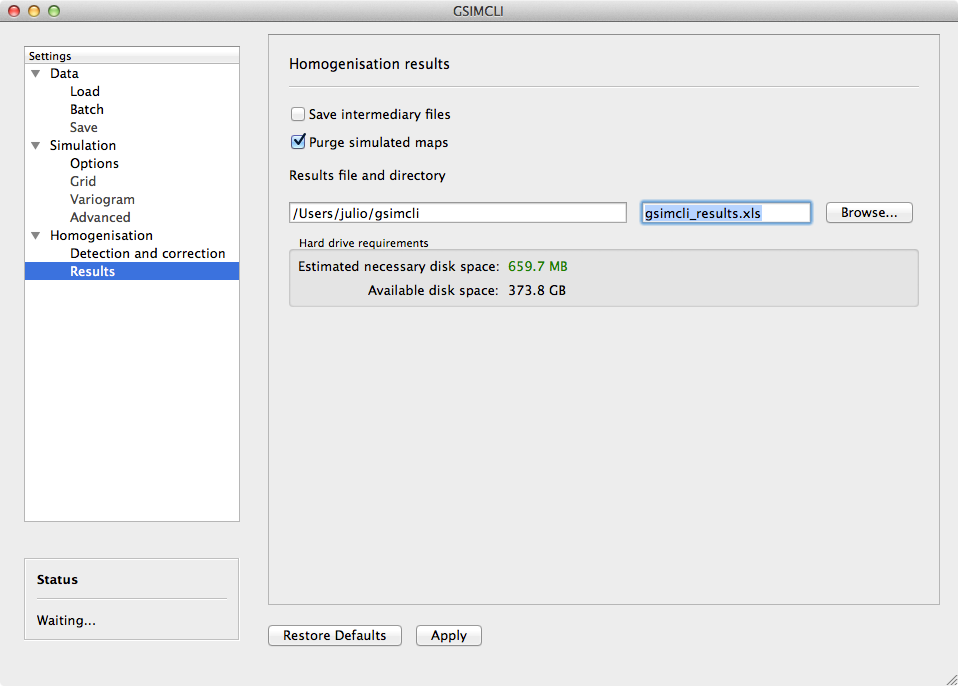
Example of the Homogenisation/Results settings pane
3.3.3.2.1. Save intermediary files
Save generated files in the procedure: intermediary PointSet files containing candidate and reference stations, homogenised and simulated values, and DSS parameters files.
If you Skip simulation and use simulated maps already in place then this option is forcibly enabled.
3.3.3.2.2. Purge simulated maps
Remove all simulated maps after the homogenisation of each candidate station. In this way, the required disk space in your computer is highly reduced, but it will not be possible to analyse the simulation results afterwards.
3.3.3.2.3. Results file and directory
Select the directory and file which will contain the homogenisation results. You can write the full directory on the left field and the file name on the right field, or you can press the Browse... button to navigate to the desired location and name the results file.
The selected directory will also be the destination folder for the intermediary and other resulting files.
If Batch networks is enabled, the Browse... button will open a
dialog for you to choose a directory (and not a file). Then you will have
to write a name for the results file on the right field. The programm will
automatically write the file extension (*.xls). Also, in this case, the
final results directory will be the selected one plus a folder with each
network name.
3.3.3.2.4. Hard drive requirements
In this area is shown the necessary and the available disk space.
The required disk space is estimated and considers only the simulated map files (the remaining files do not have a significant size). This value will be calculated (and updated) as soon as all the other settings are set up (you may have to press the Apply button to update this value).
The available disk space is shown after the results directory is selected.
In case of insufficient available disk space, please try to enable the option to Purge simulated maps. For instance, in the given example, disabling that option would increase the necessary disk space to more than 30 GB.
3.4. Bibliography
| [COSTA2009] | Costa, A., & Soares, A. (2009). Homogenization of climate data review and new perspectives using geostatistics. Mathematical Geosciences, 41(3), 291–305. doi:10.1007/s11004-008-9203-3 |